
Peak Integration
Mass spectrometry begins with a simple question: is it there?
At its core, an LC-MS/MS experiment will tell you whether a molecule is present in a sample. Each of these molecules appears as a peak on a mass chromatogram, which plots the strength of each compound’s signal over time. The process of peak detection identifies these peaks and records their mass* and retention time. This step also establishes whether the same peaks (and thus the same compounds) are detected across multiple samples. Peak detection is typically fast and, for some analyses, may be all that’s needed.
However, peaks can tell us more than just what’s there. Peaks also have areas, which can be calculated through a process called peak integration. The area under each peak reflects the relative abundance of the corresponding compound: in general, broader and taller peaks indicate higher concentrations.**
In short: peak detection tells us what’s there; peak integration tells us how much.
Understanding how much of a compound is present opens the door to all sorts of quantitative analyses that aren’t possible using peak detection alone. For example, peak detection can tell you that a compound exists in both cancer patients and healthy controls, but peak integration can tell you that it’s five times more abundant in cancer.
If you read our previous post about the differences between classical and feature-based molecular networking, you’ll know the main advantage of feature-based molecular networking is that it performs peak integration. You’ll also know that calculating these peak areas rapidly and consistently is a major challenge.

XIC?
You’ll sometimes see peak integration labeled as XIC. XIC stands for extracted ion chromatogram and refers to the process of extracting the area under the peak.
Common Issues with Peak Integration
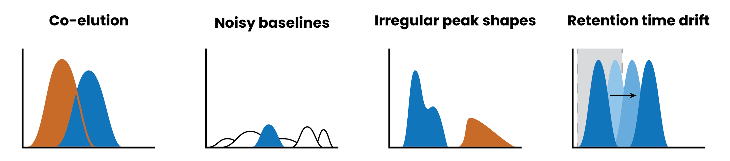
Unfortunately, accurate peak integration can be difficult. Here are some reasons why:
Co-elution
When two compounds with similar masses are measured around the same time, their peaks can overlap, making it hard to distinguish one peak from another
Noisy baselines
Poor signal-to-noise ratios can distort peak boundaries. Especially for low-abundance compounds, the signal may be indistinguishable from noise, leading to under-integration or false positives.
Irregular peak shapes
Ideally, peaks would be symmetrical and Gaussian-shaped. But in real life, peaks may tail, split, or broaden due to instrument or column issues. This can be a major hurdle for algorithms that expect pretty, symmetrical peaks.
Retention time drift:
Most peak detection and integration methods rely on retention time to determine which peaks belong to which metabolites. Unfortunately, retention time is inconsistent and can shift over the course of an experiment. If this shift isn’t corrected or retention time windows are too tight, the algorithm can miss peaks or assign them to the wrong metabolite. This is the issue behind “peak splitting”, a common problem with feature finding where a single metabolite drifts outside the retention time window over the course of the experiment, causing it to be labeled as two different metabolites.
Time
Peak integration can be one of the most computationally-intensive steps in the entire analysis process. And while waiting a few extra minutes for crucial abundance information isn’t a problem when you’re running a handful of samples, waiting three months to get that same data on a large clinical cohort is a serious issue. This is why many large metabolomics studies do not report peak area information - it’s simply too slow to run in a reasonable timeframe.
Optimizing Peak Integration
So here’s a confession - you don’t actually have to perform feature finding to get peak abundance information in Ometa Flow. One big difference between GNPS molecular networking and Ometa Flow is that we’ve built peak integration directly into our classical molecular networking, giving you the option to upload raw MS/MS data and run peak detection, peak integration, library searching, and molecular networking in a single workflow.*** While our peak integration algorithm does use retention time windows, it primarily relies on MS2 spectra to identify metabolites. MS2 tends to be more robust than retention time when comparing samples across experiments. In addition, we provide several integration options that allow users to refine parameters and even help correct for non-standard peak shapes.
While no peak integration algorithm is perfect, the ability to combine classical molecular networking and peak integration was a huge hit. It was so popular, in fact, that we soon found that the peak integration step was becoming a major computational bottleneck.
Take this molecular network of over 1,800 files. The peak integration step alone took more than 2,000 hours of compute time—over an hour per file on average.† In total, the full molecular networking workflow took over 5 days to run. (Since many of these processes are parallelized, total computational time can be higher than actual runtime).

Average and total time taken before and after optimization by the five most computationally-intensive processes in a molecular network of >1,800 samples.
After optimization, the same dataset finished in just 13 hours ‒ a 9-fold decrease in total runtime.† The peak integration step saw a 14-fold improvement, dropping from 2,000+ hours to under 150 hours of total compute time. Keen eyed figure hawks may have noticed that we also optimized the molecular networking step, but that’s a story for another day.
The best part? This analysis was run from MS/MS data directly in Ometa Flow - no having to shuffle gigabytes or even terabytes of data between tools or system file storage.
| Total Time | Total Spectra | Mean Peak Integration | Max Peak Integration | |
|---|---|---|---|---|
| Before Optimization | 5d 2h 7m 33s | 89,208 | 79.1m | 224m |
| After Optimization | 13h 31m 36s | 89,208 | 4.7m | 7.7m |
By optimizing our peak integration algorithm, we’re paving the way for high-throughput networking workflows that can provide peak detection and integration information on thousands of files in a reasonable runtime. This, combined with high-performance computing capabilities, opens the possibility of analyzing tens of thousands of MS/MS files in hours - without melting your computer.‡
Want to learn more?
* More specifically, the mass-to-charge ratio, or m/z.
**The relationship between peak area and concentration isn’t always straightforward. Read more here.
***You’re also welcome to perform peak integration with third-party tools and upload the results to our feature-based molecular networking workflow. This can even be preferred if you’ve already optimized a different peak integration tool for your data.
†Analyses were run on a local server with 20 Cores and 480GB RAM. Runtimes can be significantly improved by increasing computational resources or migrating to high performance computing (HPC).
‡Something I have definitely never done